当数据预处理完成后,我们需要选择有意义的特征输入机器学习的算法和模型进行训练。
通常来说,从两个方面考虑来选择特征:
- 特征是否发散:如果一个特征不发散,例如方差接近于0,也就是说样本在这个特征上基本上没有差异,这个特征对于样本的区分并没有什么用。
- 特征与目标的相关性:这点比较显见,与目标相关性高的特征,应当优选选择。除方差法外,本文介绍的其他方法均从相关性考虑。
特征选择主要包括:Filter Method 过滤法, Wrapper Method 包装法和Embedded Method 嵌入法。本文结合sklearn中的feature_selection库来进行特征选择的详细介绍。
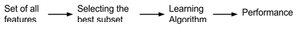
1、Filter Method 过滤法
通过统计学的方法对每个feature给出一个score, 通过score对特征进行排序,然后从中选取score最高的子集. 这种方法仅仅是对每个feature进行独立考虑,没有考虑到feature之间的依赖性或相关性. 常用的方法有: 卡方检验,信息增益等。
1.1 方差选择法
使用方差选择法,先要计算各个特征的方差,然后根据阈值,选择方差大于阈值的特征。
使用feature_selection库的VarianceThreshold类来选择特征的代码如下:
from sklearn.feature_selection import VarianceThreshold
#方差选择法,返回值为特征选择后的数据
#参数threshold为方差的阈值
VarianceThreshold(threshold=3).fit_transform(iris.data)
1.2 相关系数法
使用相关系数法,先要计算各个特征对目标值的相关系数以及相关系数的P值。
用feature_selection库的SelectKBest类结合相关系数来选择特征的代码如下:
from sklearn.feature_selection import SelectKBest
from scipy.stats import pearsonr

#选择K个最好的特征,返回选择特征后的数据
#第一个参数为计算评估特征是否好的函数,该函数输入特征矩阵和目标向量,输出二元组(评分,P值)的数组,数组第i项为第i个特征的评分和P值。在此定义为计算相关系数
#参数k为选择的特征个数
SelectKBest(lambda X, Y: array(map(lambda x:pearsonr(x, Y), X.T)).T, k=2).fit_transform(iris.data, iris.target)
1.3 卡方检验
经典的卡方检验是检验定性自变量对定性因变量的相关性。假设自变量有N种取值,因变量有M种取值,考虑自变量等于i且因变量等于j的样本频数的观察值与期望的差距,构建统计量:
这个统计量的含义简而言之就是自变量对因变量的相关性。
用feature_selection库的SelectKBest类结合卡方检验来选择特征的代码如下:
from sklearn.feature_selection import SelectKBest
from sklearn.feature_selection import chi2

#选择K个最好的特征,返回选择特征后的数据
SelectKBest(chi2, k=2).fit_transform(iris.data, iris.target)
1.4 互信息法
经典的互信息也是评价定性自变量对定性因变量的相关性的,互信息计算公式如下:

为了处理定量数据,最大信息系数法被提出,使用feature_selection库的SelectKBest类结合最大信息系数法来选择特征的代码如下:
from sklearn.feature_selection import SelectKBest
from minepy import MINE
#由于MINE的设计不是函数式的,定义mic方法将其为函数式的,返回一个二元组,二元组的第2项设置成固定的P值0.5
def mic(x, y):
m = MINE()
m.compute_score(x, y)
return (m.mic(), 0.5)
#选择K个最好的特征,返回特征选择后的数据
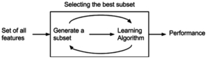
SelectKBest(lambda X, Y: array(map(lambda x:mic(x, Y), X.T)).T, k=2).fit_transform(iris.data, iris.target)2、Wrapper Method 包装法
和filter method 相比,wrapper method 考虑到了feature 之间的相关性,通过考虑feature的组合对于model性能的影响。比较不同组合之间的差异,选取性能最好的组合。比如recursive feature selection。
2.1 递归特征消除法
递归消除特征法使用一个基模型来进行多轮训练,每轮训练后,消除若干权值系数的特征,再基于新的特征集进行下一轮训练。使用feature_selection库的RFE类来选择特征的代码如下:
from sklearn.feature_selection import RFE
from sklearn.linear_model import LogisticRegression

#递归特征消除法,返回特征选择后的数据
#参数estimator为基模型
#参数n_features_to_select为选择的特征个数
RFE(estimator=LogisticRegression(), n_features_to_select=2).fit_transform(iris.data, iris.target)
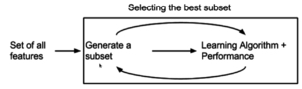
3、Embedded Method 嵌入法
结合前面二者的优点, 在模型建立的时候,同时计算模型的准确率. 最常见的embedded method 是 regularization methods(简单来说就是通过增加penalization coefficients来约束模型的复杂度)。
3.1 基于惩罚项的特征选择法
使用带惩罚项的基模型,除了筛选出特征外,同时也进行了降维。使用feature_selection库的SelectFromModel类结合带L1惩罚项的逻辑回归模型,来选择特征的代码如下:
from sklearn.feature_selection import SelectFromModel
from sklearn.linear_model import LogisticRegression

#带L1惩罚项的逻辑回归作为基模型的特征选择
SelectFromModel(LogisticRegression(penalty="l1", C=0.1)).fit_transform(iris.data, iris.target)
L1惩罚项降维的原理在于保留多个对目标值具有同等相关性的特征中的一个,所以没选到的特征不代表不重要。故,可结合L2惩罚项来优化。具体操作为:若一个特征在L1中的权值为1,选择在L2中权值差别不大且在L1中权值为0的特征构成同类集合,将这一集合中的特征平分L1中的权值,故需要构建一个新的逻辑回归模型:
from sklearn.linear_model import LogisticRegression

class LR(LogisticRegression):
    def __init__(self, threshold=0.01, dual=False, tol=1e-4, C=1.0,
                 fit_intercept=True, intercept_scaling=1, class_weight=None,
                 random_state=None, solver='liblinear', max_iter=100,
                 multi_class='ovr', verbose=0, warm_start=False, n_jobs=1):

        #权值相近的阈值
        self.threshold = threshold
        LogisticRegression.__init__(self, penalty='l1', dual=dual, tol=tol, C=C,
                 fit_intercept=fit_intercept, intercept_scaling=intercept_scaling, class_weight=class_weight,
                 random_state=random_state, solver=solver, max_iter=max_iter,
                 multi_class=multi_class, verbose=verbose, warm_start=warm_start, n_jobs=n_jobs)
        #使用同样的参数创建L2逻辑回归
        self.l2 = LogisticRegression(penalty='l2', dual=dual, tol=tol, C=C, fit_intercept=fit_intercept, intercept_scaling=intercept_scaling, class_weight = class_weight, random_state=random_state, solver=solver, max_iter=max_iter, multi_class=multi_class, verbose=verbose, warm_start=warm_start, n_jobs=n_jobs)

    def fit(self, X, y, sample_weight=None):
        #训练L1逻辑回归
        super(LR, self).fit(X, y, sample_weight=sample_weight)
        self.coef_old_ = self.coef_.copy()
        #训练L2逻辑回归
        self.l2.fit(X, y, sample_weight=sample_weight)

        cntOfRow, cntOfCol = self.coef_.shape
        #权值系数矩阵的行数对应目标值的种类数目
        for i in range(cntOfRow):
            for j in range(cntOfCol):
                coef = self.coef_[i][j]
                #L1逻辑回归的权值系数不为0
                if coef != 0:
                    idx = [j]
                    #对应在L2逻辑回归中的权值系数
                    coef1 = self.l2.coef_[i][j]
                    for k in range(cntOfCol):
                        coef2 = self.l2.coef_[i][k]
                        #在L2逻辑回归中,权值系数之差小于设定的阈值,且在L1中对应的权值为0
                        if abs(coef1-coef2) < self.threshold and j != k and self.coef_[i][k] == 0:
                            idx.append(k)
                    #计算这一类特征的权值系数均值
                    mean = coef / len(idx)
                    self.coef_[i][idx] = mean
        return self
使用feature_selection库的SelectFromModel类结合带L1以及L2惩罚项的逻辑回归模型,来选择特征的代码如下:
from sklearn.feature_selection import SelectFromModel

#带L1和L2惩罚项的逻辑回归作为基模型的特征选择
#参数threshold为权值系数之差的阈值
SelectFromModel(LR(threshold=0.5, C=0.1)).fit_transform(iris.data, iris.target)
3.2 基于树模型的特征选择法
树模型中GBDT也可用来作为基模型进行特征选择,使用feature_selection库的SelectFromModel类结合GBDT模型,来选择特征的代码如下:
from sklearn.feature_selection import SelectFromModel
from sklearn.ensemble import GradientBoostingClassifier

#GBDT作为基模型的特征选择
SelectFromModel(GradientBoostingClassifier()).fit_transform(iris.data, iris.target)
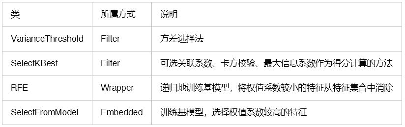
4、sklearn数据包相关类功能整理
参考:
https://blog.csdn.net/Lee20093905/article/details/79397803
https://www.cnblogs.com/jasonfreak/p/5448385.html
本文转自:博客园 - EO_Admin,转载此文目的在于传递更多信息,版权归原作者所有。


