我们在训练和验证模型时都会将训练指标保存成起来制作成图表,这样可以在结束后进行查看和分析,但是你真的了解这些指标的图表的含义吗?
在本文中将对训练和验证可能产生的情况进行总结并介绍这些图表到底能为我们提供什么样的信息。
让我们从一些简单的代码开始,以下代码建立了一个基本的训练流程框架。
from sklearn.model_selection import train_test_split
from sklearn.datasets import make_classification
import torch
from torch.utils.data import Dataset, DataLoader
import torch.optim as torch_optim
import torch.nn as nn
import torch.nn.functional as F
import numpy as np
import matplotlib.pyplot as pltclass MyCustomDataset(Dataset):
  def __init__(self, X, Y, scale=False):
      self.X = torch.from_numpy(X.astype(np.float32))
      self.y = torch.from_numpy(Y.astype(np.int64))

  def __len__(self):
      return len(self.y)

  def __getitem__(self, idx):
      return self.X[idx], self.y[idx]def get_optimizer(model, lr=0.001, wd=0.0):
  parameters = filter(lambda p: p.requires_grad, model.parameters())
  optim = torch_optim.Adam(parameters, lr=lr, weight_decay=wd)
  return optimdef train_model(model, optim, train_dl, loss_func):
  # Ensure the model is in Training mode
  model.train()
  total = 0
  sum_loss = 0
  for x, y in train_dl:
      batch = y.shape[0]
      # Train the model for this batch worth of data
      logits = model(x)
      # Run the loss function. We will decide what this will be when we call our Training Loop
      loss = loss_func(logits, y)
      # The next 3 lines do all the PyTorch back propagation goodness
      optim.zero_grad()
      loss.backward()
      optim.step()
      # Keep a running check of our total number of samples in this epoch
      total += batch
      # And keep a running total of our loss
      sum_loss += batch*(loss.item())
  return sum_loss/total
def train_loop(model, train_dl, valid_dl, epochs, loss_func, lr=0.1, wd=0):
  optim = get_optimizer(model, lr=lr, wd=wd)
  train_loss_list = []
  val_loss_list = []
  acc_list = []
  for i in range(epochs):
      loss = train_model(model, optim, train_dl, loss_func)
      # After training this epoch, keep a list of progress of
      # the loss of each epoch
      train_loss_list.append(loss)
      val, acc = val_loss(model, valid_dl, loss_func)
      # Likewise for the validation loss and accuracy
      val_loss_list.append(val)
      acc_list.append(acc)
      print("training loss: %.5f     valid loss: %.5f     accuracy: %.5f" % (loss, val, acc))

  return train_loss_list, val_loss_list, acc_list
def val_loss(model, valid_dl, loss_func):
  # Put the model into evaluation mode, not training mode
  model.eval()
  total = 0
  sum_loss = 0
  correct = 0
  batch_count = 0
  for x, y in valid_dl:
      batch_count += 1
      current_batch_size = y.shape[0]
      logits = model(x)
      loss = loss_func(logits, y)
      sum_loss += current_batch_size*(loss.item())
      total += current_batch_size
      # All of the code above is the same, in essence, to
      # Training, so see the comments there
      # Find out which of the returned predictions is the loudest
      # of them all, and that's our prediction(s)
      preds = logits.sigmoid().argmax(1)
      # See if our predictions are right
      correct += (preds == y).float().mean().item()
  return sum_loss/total, correct/batch_count
def view_results(train_loss_list, val_loss_list, acc_list):
  plt.rcParams["figure.figsize"] = (15, 5)
  plt.figure()
  epochs = np.arange(0, len(train_loss_list))   plt.subplot(1, 2, 1)
  plt.plot(epochs-0.5, train_loss_list)
  plt.plot(epochs, val_loss_list)
  plt.title('model loss')
  plt.ylabel('loss')
  plt.xlabel('epoch')
  plt.legend(['train', 'val', 'acc'], loc = 'upper left')

  plt.subplot(1, 2, 2)
  plt.plot(acc_list)
  plt.title('accuracy')
  plt.ylabel('accuracy')
  plt.xlabel('epoch')
  plt.legend(['train', 'val', 'acc'], loc = 'upper left')
  plt.show()

def get_data_train_and_show(model, batch_size=128, n_samples=10000, n_classes=2, n_features=30, val_size=0.2, epochs=20, lr=0.1, wd=0, break_it=False):
  # We'll make a fictitious dataset, assuming all relevant
  # EDA / Feature Engineering has been done and this is our
  # resultant data
  X, y = make_classification(n_samples=n_samples, n_classes=n_classes, n_features=n_features, n_informative=n_features, n_redundant=0, random_state=1972)

  if break_it: # Specifically mess up the data
      X = np.random.rand(n_samples,n_features)
  X_train, X_val, y_train, y_val = train_test_split(X, y, test_size=val_size, random_state=1972)   train_ds = MyCustomDataset(X_train, y_train)
  valid_ds = MyCustomDataset(X_val, y_val)
  train_dl = DataLoader(train_ds, batch_size=batch_size, shuffle=True)
  valid_dl = DataLoader(valid_ds, batch_size=batch_size, shuffle=True)   train_loss_list, val_loss_list, acc_list = train_loop(model, train_dl, valid_dl, epochs=epochs, loss_func=F.cross_entropy, lr=lr, wd=wd)
  view_results(train_loss_list, val_loss_list, acc_list)
以上的代码很简单,就是获取数据,训练,验证这样一个基本的流程,下面我们开始进入正题。
场景 1 - 模型似乎可以学习,但在验证或准确性方面表现不佳
无论超参数如何,模型 Train loss 都会缓慢下降,但 Val loss 不会下降,并且其 Accuracy 并不表明它正在学习任何东西。
比如在这种情况下,二进制分类的准确率徘徊在 50% 左右。
class Scenario_1_Model_1(nn.Module):
  def __init__(self, in_features=30, out_features=2):
      super().__init__()
      self.lin1 = nn.Linear(in_features, out_features)
  def forward(self, x):
      x = self.lin1(x)
      return x

get_data_train_and_show(Scenario_1_Model_1(), lr=0.001, break_it=True)
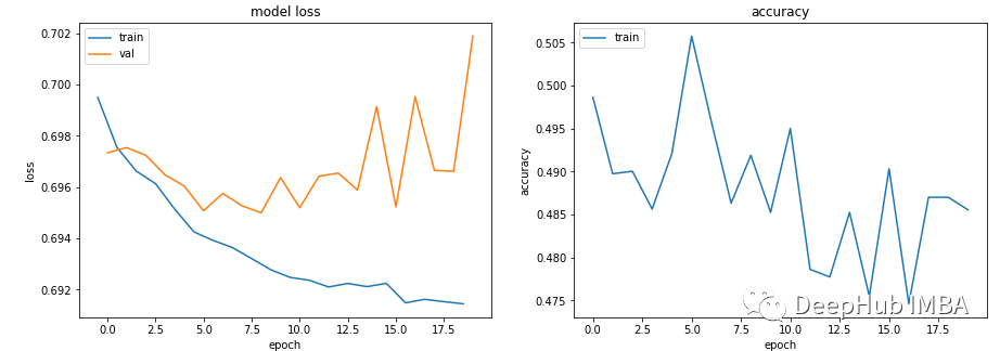
数据中没有足够的信息来允许‘学习’,训练数据可能没有包含足够的信息来让模型“学习”。
在这种情况下(代码中训练数据是随机数据),这意味着它无法学习任何实质内容。
数据必须有足够的信息可以从中学习。EDA 和特征工程是关键!模型学习可以学到的东西,而不是不是编造不存在的东西。
场景 2 — 训练、验证和准确度曲线都非常不稳
例如下面代码:lr=0.1,bs=128
class Scenario_2_Model_1(nn.Module):
  def __init__(self, in_features=30, out_features=2):
      super().__init__()
      self.lin1 = nn.Linear(in_features, out_features)
  def forward(self, x):
      x = self.lin1(x)
      return x

get_data_train_and_show(Scenario_2_Model_1(), lr=0.1)
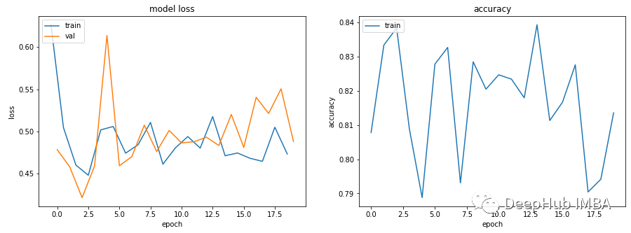
“学习率太高”或“批量太小”可以尝试将学习率从 0.1 降低到 0.001,这意味着它不会“反弹”,而是会平稳地降低。
get_data_train_and_show(Scenario_1_Model_1(), lr=0.001)
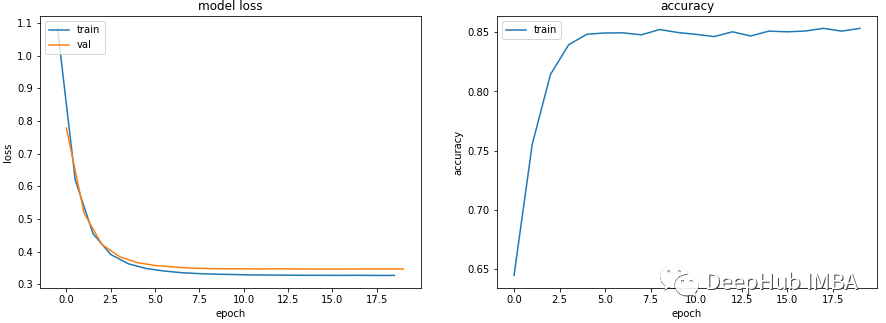
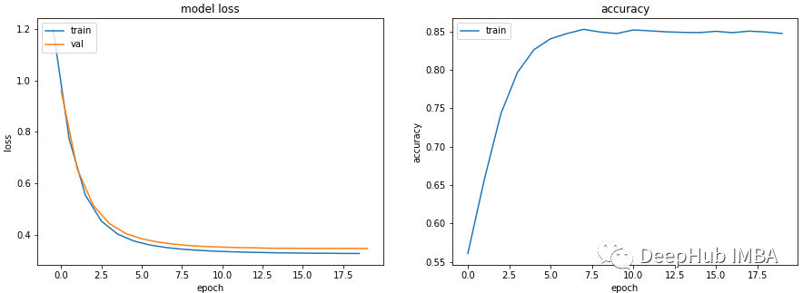
除了降低学习率外,增加批量大小也会使其更平滑。
get_data_train_and_show(Scenario_1_Model_1(), lr=0.001, batch_size=256)
场景 3——训练损失接近于零,准确率看起来还不错,但验证 并没有下降,并且还上升了
class Scenario_3_Model_1(nn.Module):
  def __init__(self, in_features=30, out_features=2):
      super().__init__()
      self.lin1 = nn.Linear(in_features, 50)
      self.lin2 = nn.Linear(50, 150)
      self.lin3 = nn.Linear(150, 50)
      self.lin4 = nn.Linear(50, out_features)
  def forward(self, x):
      x = F.relu(self.lin1(x))
      x = F.relu(self.lin2(x))
      x = F.relu(self.lin3(x))
      x = self.lin4(x)
      return x
get_data_train_and_show(Scenario_3_Model_1(), lr=0.001)
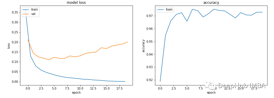
这肯定是过拟合了:训练损失低和准确率高,而验证损失和训练损失越来越大,都是经典的过拟合指标。
从根本上说,你的模型学习能力太强了。它对训练数据的记忆太好,这意味着它也不能泛化到新数据。
我们可以尝试的第一件事是降低模型的复杂性。
class Scenario_3_Model_2(nn.Module):
  def __init__(self, in_features=30, out_features=2):
      super().__init__()
      self.lin1 = nn.Linear(in_features, 50)
      self.lin2 = nn.Linear(50, out_features)
  def forward(self, x):
      x = F.relu(self.lin1(x))
      x = self.lin2(x)
      return x

get_data_train_and_show(Scenario_3_Model_2(), lr=0.001)
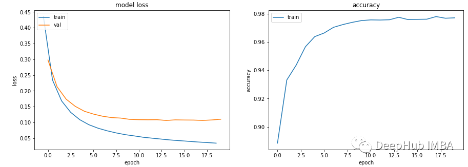
这让它变得更好了,还可以引入 L2 权重衰减正则化,让它再次变得更好(适用于较浅的模型)。
get_data_train_and_show(Scenario_3_Model_2(), lr=0.001, wd=0.02)
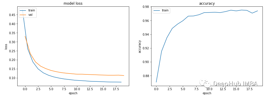
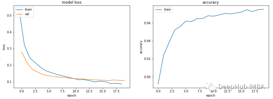
如果我们想保持模型的深度和大小,可以尝试使用 dropout(适用于更深的模型)。
class Scenario_3_Model_3(nn.Module):
  def __init__(self, in_features=30, out_features=2):
      super().__init__()
      self.lin1 = nn.Linear(in_features, 50)
      self.lin2 = nn.Linear(50, 150)
      self.lin3 = nn.Linear(150, 50)
      self.lin4 = nn.Linear(50, out_features)
      self.drops = nn.Dropout(0.4)
  def forward(self, x):
      x = F.relu(self.lin1(x))
      x = self.drops(x)
      x = F.relu(self.lin2(x))
      x = self.drops(x)
      x = F.relu(self.lin3(x))
      x = self.drops(x)
      x = self.lin4(x)
      return x
get_data_train_and_show(Scenario_3_Model_3(), lr=0.001)
场景 4 - 训练和验证表现良好,但准确度没有提高
lr = 0.001,bs = 128(默认,分类类别= 5
class Scenario_4_Model_1(nn.Module):
  def __init__(self, in_features=30, out_features=2):
      super().__init__()
      self.lin1 = nn.Linear(in_features, 2)
      self.lin2 = nn.Linear(2, out_features)
  def forward(self, x):
      x = F.relu(self.lin1(x))
      x = self.lin2(x)
      return x

get_data_train_and_show(Scenario_4_Model_1(out_features=5), lr=0.001, n_classes=5)
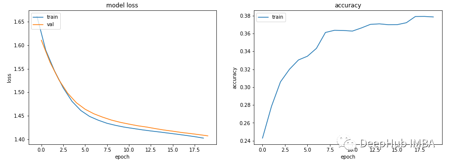
没有足够的学习能力:模型中的其中一层的参数少于模型可能输出中的类。在这种情况下,当有 5 个可能的输出类时,中间的参数只有 2 个。
这意味着模型会丢失信息,因为它不得不通过一个较小的层来填充它,因此一旦层的参数再次扩大,就很难恢复这些信息。
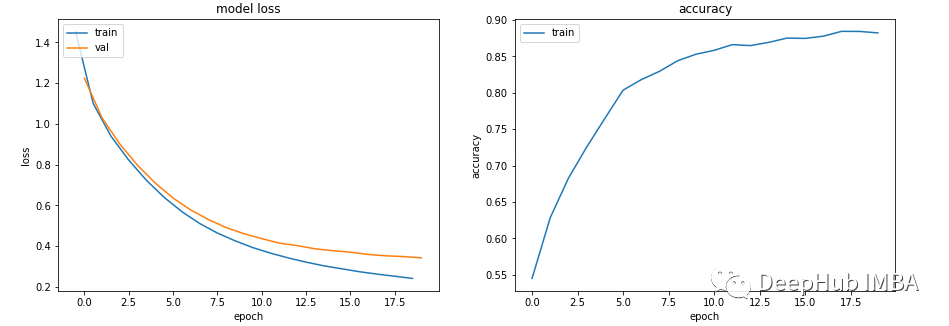
所以需要记录层的参数永远不要小于模型的输出大小。
class Scenario_4_Model_2(nn.Module):
  def __init__(self, in_features=30, out_features=2):
      super().__init__()
      self.lin1 = nn.Linear(in_features, 50)
      self.lin2 = nn.Linear(50, out_features)
  def forward(self, x):
      x = F.relu(self.lin1(x))
      x = self.lin2(x)
      return x
get_data_train_and_show(Scenario_4_Model_2(out_features=5), lr=0.001, n_classes=5)
总结
以上就是一些常见的训练、验证时的曲线的示例,希望你在遇到相同情况时可以快速定位并且改进。
作者:Martin Keywood
声明:本文为转载文章,转载此文目的在于传递更多信息,版权归原作者所有,如涉及侵权,请联系小编邮箱 demi@eetrend.com 进行处理。