LSTM原理及实现（二）

上一篇：LSTM原理及实现（一）

作者：bill_b

在一篇中着核心要素简述了LSTM算法的原理，本篇中将在本人做过一些前置处理的数据集上实现LSTM的一个实际应用案例。该数据集是一段时间内的时序数据，数据做过脱敏处理，列特征标识为A,B,C，其三者间存在一点关系影响，本案例将基于LSTM算法实现多变量时间序列的重构+预测。

数据集：https://download.csdn.net/download/weixin_44162104/11200183

完整代码：https://github.com/521bibi/LSTMdemo

数据读取

class XLSReader(object):
    def __init__(self):
        file  = 'E:\pyProjects\LSTMdemo\data\LSTMdemo.xlsx'
        self.xls_read = pd.read_excel(file,header=None,parse_dates=[0])

    def read(self):
        xls_data = self.xls_read
        parse_data = self.parse_xls(xls_data)
        return parse_data

    def parse_xls(self,content):
        parse_data = content.iloc[1:,:4]
        # parse_data[0] = pd.to_datetime(parse_data[0], format="%Y/%m/%d %H:%M:%S")
        parse_data.set_index(0, inplace=True)
        return parse_data

构建Excel读取函数XLSReader，读取目标数据集，将第一列时间轴数据作为行名，A,B,C作为列名。

reader = XLSReader()
df_result = reader.read()
print(df_result)

数据预处理

缺省值处理

values = df_result.values
# ensure all data is float
values = values.astype('float32')
# normalize features
scaler = MinMaxScaler(feature_range=(0, 1))
scaled = scaler.fit_transform(values)

归一化处理

values = df_result.values
# ensure all data is float
values = values.astype('float32')
# normalize features
scaler = MinMaxScaler(feature_range=(0, 1))
scaled = scaler.fit_transform(values)

建模训练

输入

# split into train and test sets
splitpoint = 450
train = scaled[:splitpoint,:]
test = scaled[splitpoint:,:]

将数据集切分为训练集和验证集

# split into input and output
train_X,train_y = train[:-1,:3],train[1:,0]
test_X, test_y = test[:-1, :3], test[1:, 0]

以A,B,C作为特征输入，预测下一时刻的A列数据。本例demo只对A列数据做重构，其余两列基本一模一样。

# reshape input to be 3D(samples,timesteps,features)
train_X = train_X.reshape(train_X.shape[0],1,train_X.shape[1])
test_X = test_X.reshape(test_X.shape[0], 1, test_X.shape[1])
# print(self.train_X.shape,self.train_y.shape,test_X.shape,test_y.shape)

将输入转为Keras中LSTM的API的标准输入格式，第二维设置为1是设置本例的LSTM步长为1，上一时刻对下一时刻的预测，对数据集的观测，我们可以知道以天为周期同样存在很强关系，设置步长为24的训练结果可以与此对比，哪种模型更佳。（本例旨在介绍LSTM的实例应用，在此不做对比了）

模型搭建

# design network
model = Sequential()
# model.add(LSTM(10, input_shape=(train_X.shape[1], train_X.shape[2])))
model.add(LSTM(4, input_shape=(train_X.shape[1], train_X.shape[2]),return_sequences=True))
model.add(LSTM(4, return_sequences=False))
model.add(Dense(1))
model.compile(loss='mae', optimizer='adam')

通过多次人工试验，建立了两层LSTM结构，第一层和第二层都设置的4个LSTMcell单元，代价函数采用mae，优化器采用adam算法。

模型训练和保存

# fit network
history = model.fit(train_X, train_y, nb_epoch=20, batch_size=1,validation_data=(test_X, test_y), verbose=2,shuffle=False)
model.save("currentlstm.h5")
#plot history
plt.plot(history.history['loss'],label='train')
plt.plot(history.history['val_loss'], label='test')
plt.legend()
plt.show()

拟合效果

plt.figure(figsize=(16,8))
train_predict = model.predict(train_X)
test_predict = model.predict(test_X)
plt.plot(scaled[1:,0], c='b')
plt.plot([x for x in train_predict], c='g')
plt.plot([None for _ in train_predict] + [x for x in test_predict], c='y')
plt.show()

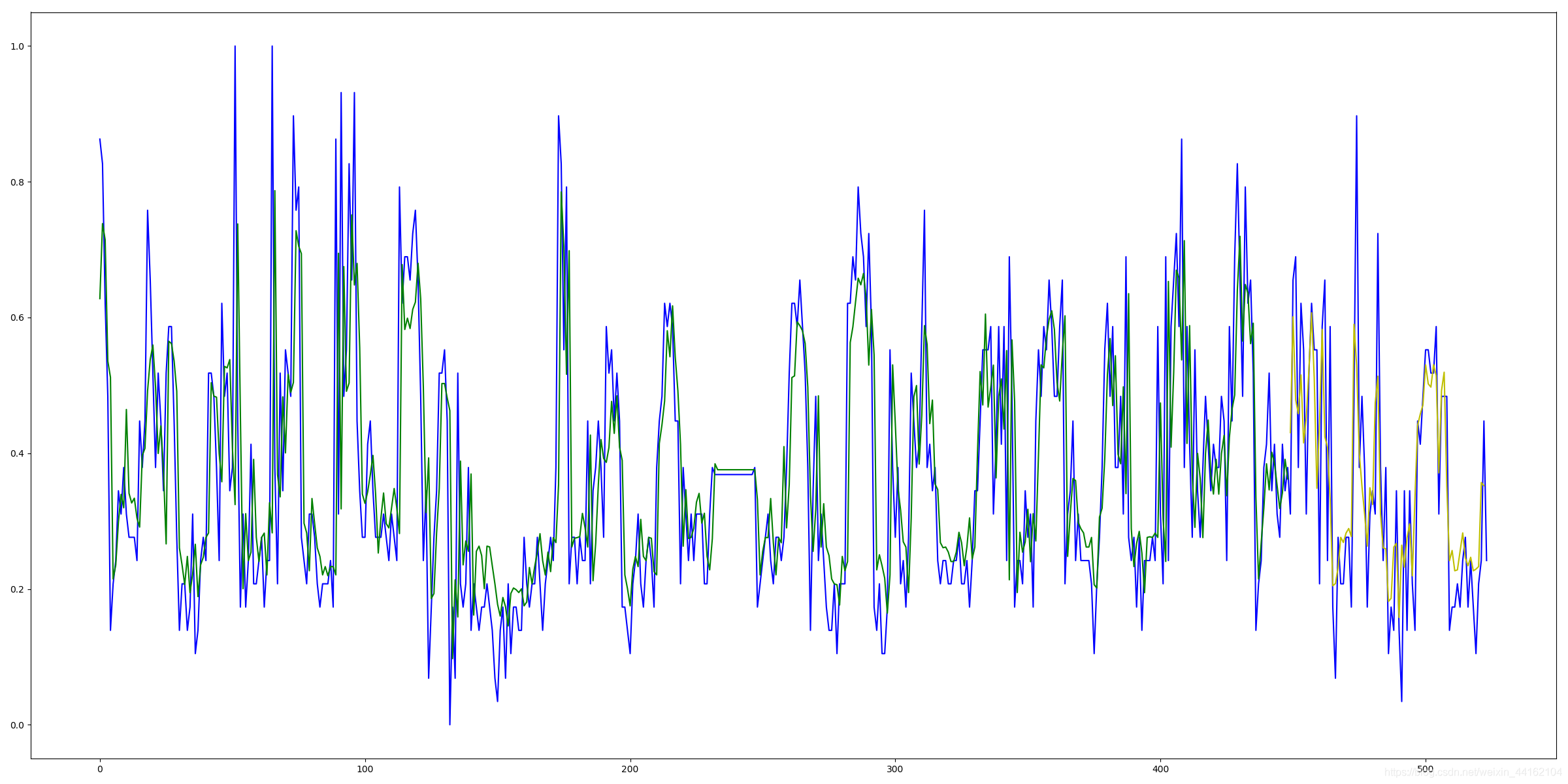
归一化数据集上的拟合效果，其中绿色为训练集拟合效果，黄色是验证集。

模型应用和预测

数据重构

#download model
model = load_model('currentlstm.h5')

plt.figure(figsize=(24,12))
current_predict = model.predict(current_X)

归一化反转

# 归一化反转
from numpy import concatenate
# invert scaling for forecast
inv_yhat = concatenate((currentA_predict,currentB_predict,currentC_predict), axis=1)
current_X = inv_yhat
inv_yhat = scaler.inverse_transform(inv_yhat)

预测

for i in range(12):
    # reshape input to be 3D(samples,timesteps,features)
    current_X = current_X.reshape(current_X.shape[0],1,current_X.shape[1])

    #download model
    model = load_model('currentlstm.h5')
    currentA_predict = model.predict(current_X)
    # print(currentA_predict)

    model = load_model('currentB_lstm.h5')
    currentB_predict = model.predict(current_X)
    # print(currentB_predict)

    model = load_model('currentC_lstm.h5')
    currentC_predict = model.predict(current_X)
    # print(currentC_predict)

    # 归一化反转
    from numpy import concatenate
    # invert scaling for forecast
    inv_yhat = concatenate((currentA_predict,currentB_predict,currentC_predict), axis=1)
    current_X = inv_yhat
    inv_yhat = scaler.inverse_transform(inv_yhat)
    # print(inv_yhat)
    current_predict = np.row_stack((current_predict, inv_yhat))
    # print("%d:"%i,current_X)
    print('数据处理中: {:.2%}'.format((i+1) /12))

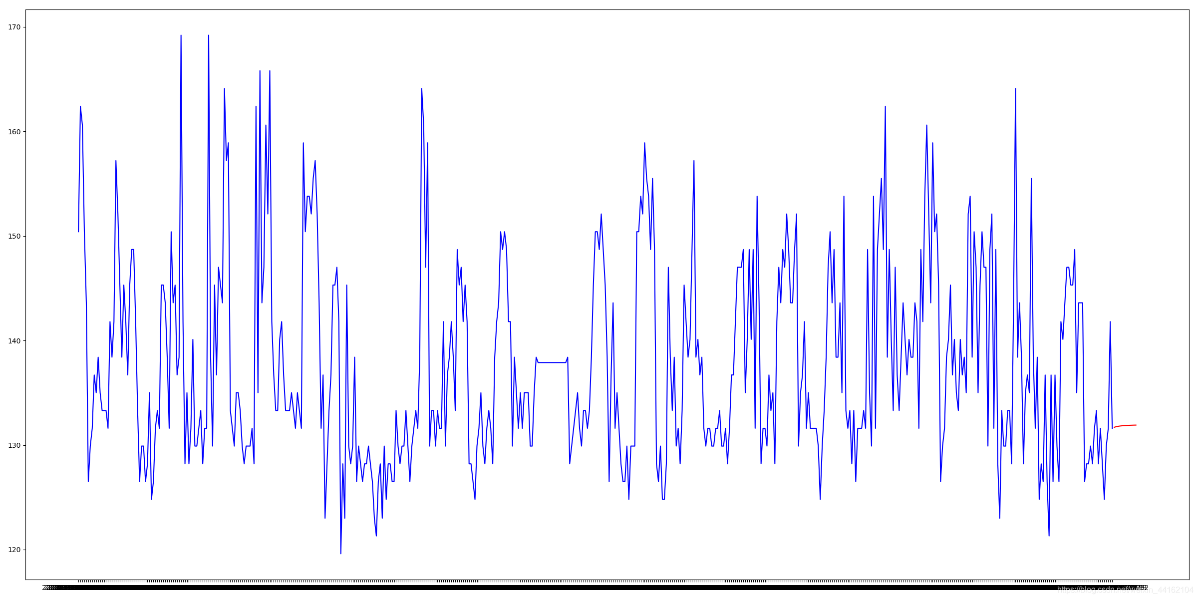
此前本人已经对数据集的A,B,C三个时序的模型训练调试了多次，最终择优确定了模型，在此demo中就忽略了其他两列数据的模型训练，方法和对A类似，只是得到的模型结构和参数不一致。

预测采用循环滚动的预测方式，我们要预测未来12个小时的时序值，模型每次输入为上一时刻A,B,C三个数据，因此要不停滚动得到每一个时刻的三项数据。

版权声明：本文为CSDN博主「bill_b」的原创文章，遵循CC 4.0 BY-SA版权协议，转载请附上原文出处链接及本声明。
原文链接：https://blog.csdn.net/weixin_44162104/article/details/90515372