很多正在入门或刚入门TensorFlow机器学习的同学希望能够通过自己指定图片源对模型进行训练,然后识别和分类自己指定的图片。但是,在TensorFlow官方入门教程中,并无明确给出如何把自定义数据输入训练模型的方法。现在,我们就参考官方入门课程《Deep MNIST for Experts》一节的内容(传送门: https://www.tensorflow.org/get_started/mnist/pros ),介绍如何将自定义图片输入到TensorFlow的训练模型。
在《Deep MNISTfor Experts》一节的代码中,程序将TensorFlow自带的mnist图片数据集mnist.train.images作为训练输入,将mnist.test.images作为验证输入。当学习了该节内容后,我们会惊叹卷积神经网络的超高识别率,但对于刚开始学习TensorFlow的同学,内心可能会产生一个问号:如何将mnist数据集替换为自己指定的图片源?譬如,我要将图片源改为自己C盘里面的图片,应该怎么调整代码?
我们先看下该节课程中涉及到mnist图片调用的代码:
from tensorflow.examples.tutorials.mnist import input_data
mnist = input_data.read_data_sets('MNIST_data', one_hot=True)
batch = mnist.train.next_batch(50)
train_accuracy = accuracy.eval(feed_dict={x: batch[0], y_: batch[1], keep_prob: 1.0})
train_step.run(feed_dict={x: batch[0], y_: batch[1], keep_prob: 0.5})
print('test accuracy %g' % accuracy.eval(feed_dict={x: mnist.test.images, y_: mnist.test.labels, keep_prob: 1.0}))
对于刚接触TensorFlow的同学,要修改上述代码,可能会较为吃力。我也是经过一番摸索,才成功调用自己的图片集。
要实现输入自定义图片,需要自己先准备好一套图片集。为节省时间,我们把mnist的手写体数字集一张一张地解析出来,存放到自己的本地硬盘,保存为bmp格式,然后再把本地硬盘的手写体图片一张一张地读取出来,组成集合,再输入神经网络。mnist手写体数字集的提取方式详见《如何从TensorFlow的mnist数据集导出手写体数字图片》。
将mnist手写体数字集导出图片到本地后,就可以仿照以下python代码,实现自定义图片的训练:
#!/usr/bin/python3.5
# -*- coding: utf-8 -*-
import os
import numpy as np
import tensorflow as tf
from PIL import Image
# 第一次遍历图片目录是为了获取图片总数
input_count = 0
for i in range(0,10):
dir = './custom_images/%s/' % i # 这里可以改成你自己的图片目录,i为分类标签
for rt, dirs, files in os.walk(dir):
for filename in files:
input_count += 1
# 定义对应维数和各维长度的数组
input_images = np.array([[0]*784 for i in range(input_count)])
input_labels = np.array([[0]*10 for i in range(input_count)])
# 第二次遍历图片目录是为了生成图片数据和标签
index = 0
for i in range(0,10):
dir = './custom_images/%s/' % i # 这里可以改成你自己的图片目录,i为分类标签
for rt, dirs, files in os.walk(dir):
for filename in files:
filename = dir + filename
img = Image.open(filename)
width = img.size[0]
height = img.size[1]
for h in range(0, height):
for w in range(0, width):
# 通过这样的处理,使数字的线条变细,有利于提高识别准确率
if img.getpixel((w, h)) > 230:
input_images[index][w+h*width] = 0
else:
input_images[index][w+h*width] = 1
input_labels[index][i] = 1
index += 1
# 定义输入节点,对应于图片像素值矩阵集合和图片标签(即所代表的数字)
x = tf.placeholder(tf.float32, shape=[None, 784])
y_ = tf.placeholder(tf.float32, shape=[None, 10])
x_image = tf.reshape(x, [-1, 28, 28, 1])
# 定义第一个卷积层的variables和ops
W_conv1 = tf.Variable(tf.truncated_normal([7, 7, 1, 32], stddev=0.1))
b_conv1 = tf.Variable(tf.constant(0.1, shape=[32]))
L1_conv = tf.nn.conv2d(x_image, W_conv1, strides=[1, 1, 1, 1], padding='SAME')
L1_relu = tf.nn.relu(L1_conv + b_conv1)
L1_pool = tf.nn.max_pool(L1_relu, ksize=[1, 2, 2, 1], strides=[1, 2, 2, 1], padding='SAME')
# 定义第二个卷积层的variables和ops
W_conv2 = tf.Variable(tf.truncated_normal([3, 3, 32, 64], stddev=0.1))
b_conv2 = tf.Variable(tf.constant(0.1, shape=[64]))
L2_conv = tf.nn.conv2d(L1_pool, W_conv2, strides=[1, 1, 1, 1], padding='SAME')
L2_relu = tf.nn.relu(L2_conv + b_conv2)
L2_pool = tf.nn.max_pool(L2_relu, ksize=[1, 2, 2, 1], strides=[1, 2, 2, 1], padding='SAME')
# 全连接层
W_fc1 = tf.Variable(tf.truncated_normal([7 * 7 * 64, 1024], stddev=0.1))
b_fc1 = tf.Variable(tf.constant(0.1, shape=[1024]))
h_pool2_flat = tf.reshape(L2_pool, [-1, 7*7*64])
h_fc1 = tf.nn.relu(tf.matmul(h_pool2_flat, W_fc1) + b_fc1)
# dropout
keep_prob = tf.placeholder(tf.float32)
h_fc1_drop = tf.nn.dropout(h_fc1, keep_prob)
# readout层
W_fc2 = tf.Variable(tf.truncated_normal([1024, 10], stddev=0.1))
b_fc2 = tf.Variable(tf.constant(0.1, shape=[10]))
y_conv = tf.matmul(h_fc1_drop, W_fc2) + b_fc2
# 定义优化器和训练op
cross_entropy = tf.reduce_mean(tf.nn.softmax_cross_entropy_with_logits(labels=y_, logits=y_conv))
train_step = tf.train.AdamOptimizer((1e-4)).minimize(cross_entropy)
correct_prediction = tf.equal(tf.argmax(y_conv, 1), tf.argmax(y_, 1))
accuracy = tf.reduce_mean(tf.cast(correct_prediction, tf.float32))
with tf.Session() as sess:
sess.run(tf.global_variables_initializer())
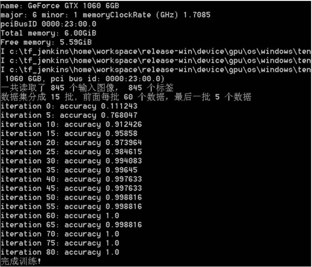
print ("一共读取了 %s 个输入图像, %s 个标签" % (input_count, input_count))
# 设置每次训练op的输入个数和迭代次数,这里为了支持任意图片总数,定义了一个余数remainder,譬如,如果每次训练op的输入个数为60,图片总数为150张,则前面两次各输入60张,最后一次输入30张(余数30)
batch_size = 60
iterations = 100
batches_count = int(input_count / batch_size)
remainder = input_count % batch_size
print ("数据集分成 %s 批, 前面每批 %s 个数据,最后一批 %s 个数据" % (batches_count+1, batch_size, remainder))
# 执行训练迭代
for it in range(iterations):
# 这里的关键是要把输入数组转为np.array
for n in range(batches_count):
train_step.run(feed_dict={x: input_images[n*batch_size:(n+1)*batch_size], y_: input_labels[n*batch_size:(n+1)*batch_size], keep_prob: 0.5})
if remainder > 0:
start_index = batches_count * batch_size;
train_step.run(feed_dict={x: input_images[start_index:input_count-1], y_: input_labels[start_index:input_count-1], keep_prob: 0.5})
# 每完成五次迭代,判断准确度是否已达到100%,达到则退出迭代循环
iterate_accuracy = 0
if it%5 == 0:
iterate_accuracy = accuracy.eval(feed_dict={x: input_images, y_: input_labels, keep_prob: 1.0})
print ('iteration %d: accuracy %s' % (it, iterate_accuracy))
if iterate_accuracy >= 1:
break;
print ('完成训练!')
上述python代码的执行结果截图如下:
对于上述代码中与模型构建相关的代码,请查阅官方《Deep MNIST for Experts》一节的内容进行理解。在本文中,需要重点掌握的是如何将本地图片源整合成为feed_dict可接受的格式。其中最关键的是这两行:
# 定义对应维数和各维长度的数组
input_images = np.array([[0]*784 for i in range(input_count)])
input_labels = np.array([[0]*10 for i in range(input_count)])
它们对应于feed_dict的两个placeholder:
x = tf.placeholder(tf.float32, shape=[None, 784])
y_ = tf.placeholder(tf.float32, shape=[None, 10])
这样一看,是不是很简单?
出处:ShadowN1ght的博客
原文链接: https://blog.csdn.net/ShadowN1ght/article/details/78076081